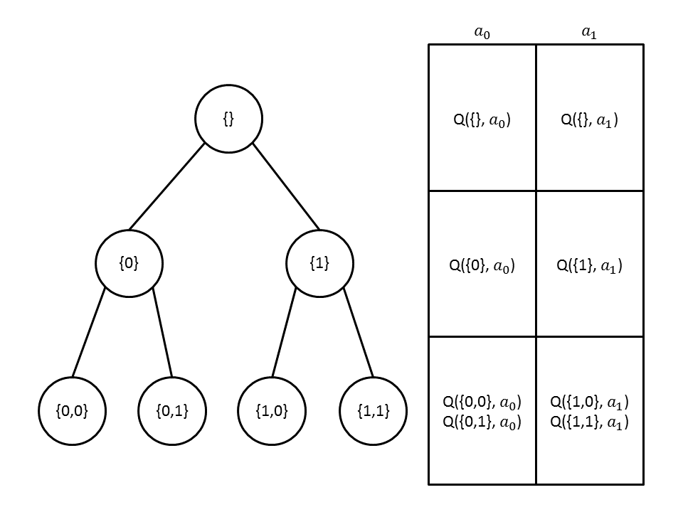
QTable Representation¶

We understand that the number of states in this problem is colossal. Henceforth, we need to be very careful how we represent the states in the Q-Table. Moreover, we recognize that we need to be diligent and careful in designing and implementing the Q-Table such that the Lookup and Update of the states and their respective Q-Value are fast. If the Q-Table is poorly implemented, the Q-Agent will perform miserably. In our algorithm, we will refer Q-Table as Q-Tree. The reason for this is because the data structure is shaped like a tree instead of a table due to the nature of our problem, refer to Figure below for a graphical representation. In this section, we will list down the 3 attempts at designing the Q-Tree. We will also discuss modifications to the state representation. We also note that in our discussions, we do not consider the complexity of the distance calculations as the complexity is the same across all data structures.

Attempt 1 - KD-Tree¶

KD-Tree is a generalized binary tree in $k$-dimentions\cite{bentley1975multidimensional}. KD-Trees are designed to address the inefficiency of the brute-force in machine learning. The tree aims to minimize the number of distance calculations by encoding aggregate distance information. The intuition is given 3 $n$-dimensional points $A,B,C$, if we know that $A$ and $C$ are very far apart and if $B$ is very close to $A$. Hence, we can automatically conclude that the $A$ and $B$ are distant, saving a distance computation. The complexity of KD-Tree for insertion, querying and deletion is the same, $\mathcal{O}(\log{n})$.

We also note that in literature, KD-Trees are not suitable for problems with high-dimensional spaces. KD-Tree is most effective when the number of points $n$ is large, more specifically when $n >> 2^k$, as it would be digressing to exhaustive search\cite{indyk2004nearest}.

Attempt 2 - Arrays¶

Arrays is a data structure storing an ordered collection of elements. In our discussion, we will reasonably assume arrays are implemented on a deterministic machine with contiguous memory block. We note that we will benefit from caching effect. Intuitively, at Henceforth, the complexity for search is $\mathcal{O}(n)$, insertion and deletion would be $\mathcal{O}(1)$, random access would be $\mathcal{O}(1)$. This is because we would need to perform a linear search over the entire array to find the closest match to any given state. Before we continue, we make a note of an important insight into Q-Learning. As the algorithm progresses, it converges to optimal. Typically, the reward value increases as time passes and the algorithm will select the same state more frequently. With this insight, we can sort the underlying array. Experimentally and intuitively, it gives us a better performance due to the higher probability of matching a given state. However, we note that the worst-case complexity is the same as the aforementioned complexity. An example is given in Figure below.

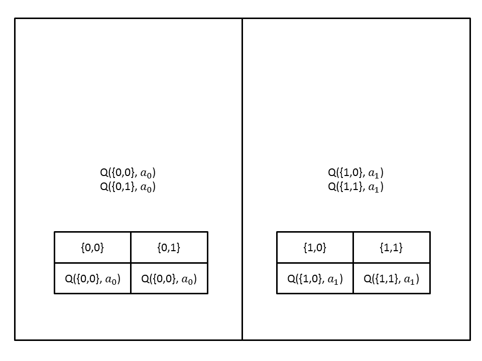
We also note that we modify the representation of the state, deviating from the representation mentioned earlier. We now give a representation that is equivalent to the one that we had mentioned in the framework. We make two adjustments to the state representation. Firstly, the new state representation will be represented as bit vectors which can be efficiently implemented on any modern machine. Secondly, we will represent the features not yet considered by the size of the bit vector. Hence, a state originally represented as $(1,0,-1,-1)$ is represented as a bit vector $10$. Similarly, $(1,0,0,0)$ is represented as $1000$. This allows us to use fast bit operations. In addition, we can use Hamming-Distance to calculate the distance of the bit vectors which can be efficiently implemented using bit operations. This would give us a major advantage compared with KD-Tree, even though the complexity for KD-Trees are better.

We will also further assume that the size of the array at each level is fixed. We make note that the size at each level is bounded by $\min(2^{m_i}, n)$, where $m_i$ is the number of features that have been considered at level $i$. From our discussion above, it should be clear that the binary vector processed at the $i$-th level must be of size $i$. Henceforth, the number of possible unique bit vectors would be $2^{m_i}$. Additionally, the number of bit vectors cannot exceed the total number of episodes that the agent performs. Assuming that the agent finds $1$ unique and new bit vector for level $i$, then it is $n$. Henceforth, we give an upper bound of the memory usage of the data structure in the equation below. We also make the reasonable assumption that $n>m$ as typical datasets the number of instances $n$ is larger than the number of features $m$.

$$ \mathcal{O}(\sum_{i=0}^{m} \min(2^{m_i}, n)) \implies \mathcal{O}(n \times m), \text{where } n > m $$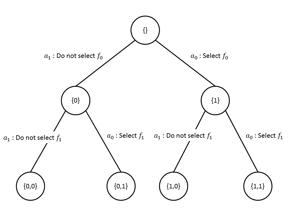

We now make another insight, deletion never happens in our array. This is because the operations that the Q-Tree performs only insert, update and search operations, updating of the Q-Value and searching for the state and its corresponding Q-Value. We also note that we know the difference $\delta = q_0 - q_1$ between the old Q-Value $q_0$ and the new $q_1$. Hence, we can update by simply performing a binary search of the value $q_1$ to the sub-array, either at the front or the back(determined by $\delta$) relative to the old position. Thereafter, we shifts all the values between the old position and the new position. However, this does not change the wose case complexity of the update operation.

Attempt 3 - Doubly Linked List¶

We recognize that all the insights in attempt 2 can be applied to the doubly linked list. The difference between the array and the link list is that the link list would avoid the shifting of the elements. Shifting elements is an expensive operation as all the $n$ elements will have to be rewritten to their adjacent cells. We also note that in this representation, we lose the ability to perform binary search because we no longer have random access of $\mathcal{O}(1)$. However, the binary search operation is not the most expensive operation but the shifting of the elements. We attempt to rectify this by using doubly linked list. We can search in the direction as determined by $\delta$ as mentioned in attempt 2 and just splice at the appropriate position. However, the worst-case complexity would be still the same, listed below. However, it would intuitively reap a performance benefit as the number of operations performed reduced, and they are less expensive.

Search: $\mathcal{O}(n)$
Update: $\mathcal{O}(n)$
Insert: $\mathcal{O}(n)$

Testing the optimizations of Q-Tree¶

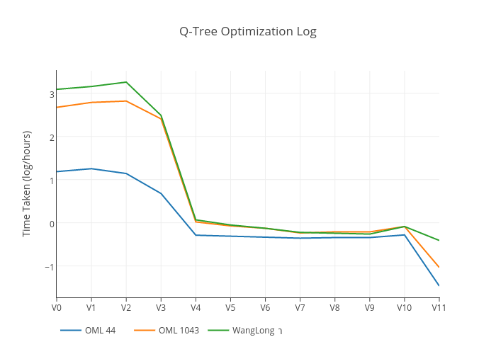
In this section, we will discuss the implementation details of the Q-Tree that we have implemented. We also make a note of the optimizations that we have performed. In this section, we have used the datasets in our preliminary testing to test the Q-Tree. Figure below shows the run times of the Fast Q Agent with default hyperparameters. We now describe briefly the optimizations done below:

Version 0: No Optimization
Version 1: Code refactoring and basic memory optimization(copying optimization, etc... )
Version 2: Architectural changes, basic optimizations
Version 3: Change of underlying data structure to numpy arrays
Version 4: Upgrade numerical computation library to use gmpy2, performing computation of Hamming Distance in C code.
Version 5: Optimize updates using functional style, without branching
Version 6: Another architecture change in Qtree, to use functional style
Version 7: Array sorted on Q-Value
Version 8: Value and copy optimizations
Version 9: Reuse state and optimized binary search
Version 10: Change data structure to Linked List
Version 11: Do not use Parallel computation in Machine Learning algorithm

Extension to using Max Trie Tree¶

Extension, not in FYP.

From Wikipedia: In computer science, a trie, also called digital tree, radix tree or prefix tree, is a kind of search tree—an ordered tree data structure used to store a dynamic set or associative array where the keys are usually strings. Unlike a binary search tree, no node in the tree stores the key associated with that node; instead, its position in the tree defines the key with which it is associated. All the descendants of a node have a common prefix of the string associated with that node, and the root is associated with the empty string. Keys tend to be associated with leaves, though some inner nodes may correspond to keys of interest. Hence, keys are not necessarily associated with every node.

We can use trie trees in 2 ways in our program:

Used as a replacement of the Q-Table, where we can find the best approximate matches by partially traversing the Trie Tree. We would store the Q values inside the Trie Tree and use the values during partial traversal
Used to store the approximate expectation of q value

First Case¶

We have not implemented the change to #1 but we think will give rise to significant performance (time) improvements. However, there will be no accuracy improvements.

Second Case¶

In the second case, we will also use a max trie tree to represent the optimal feature subset's score on the current path. We can use this optimal feature subset's score to approximate the long run Q-value for which the algorithm will converge to. We will always use this value if it is avaliable, over the estimate from the Q table.

The concept is as follows, we start with the update equation and rewrite it such that it is not in a recusive relation. We can do this because we have assume a finite horizon to the problem. We start with the q-value update equation and end up with:

$$ q_{i} = \sum_{k=0}^{N-1}{r_{i+k}\gamma^k + \gamma^{N-i}q_N} $$

In our problem, we do not apply any intermediary reward, so we can reduce the relation to:

$$ q_{i} = \sum_{k=0}^{N-1}{\gamma^{N-i}q_N} $$

Since at each $i$ we are interested in comparing the subsequent q values, we can omit the $\gamma$. Additionally, for our problem $q_N$ is just the accuraccy. In that way, we can approximate the expected action on the optimal policy to be:

$$ a = \text{argmax}_a q_{i+1,a} = \text{argmax}_a \text{reachable}(q_{N},a) $$

Hence, we can use trie tree to capture the largest possible $q_{N}$ on every path. We will use this optimization when both $q_N$ form the next action are avaliable. If the 2 values are unavaliable, we will default back to the approximation of the q-value in the traditional way.

Note on overfitting: we recognize that we will be greedily selecting the path that yield best performance. However, we will only be using this method to select the actions during training. We will not use this method at all when we are selecting a specific feature subset.

In our experiments, we observed some performance improvements for smaller feature spaces.